Mark Bauman | Endurica LLC

Road Loads to Block Cycle Schedule

June 9, 2022March 12, 2021 by Mark Bauman

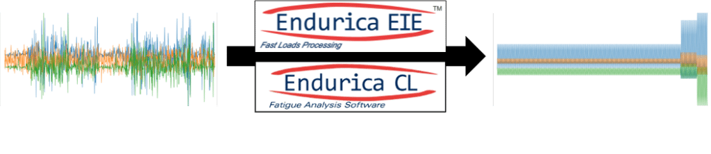
Road loads being converted into block cycle schedules through Endurica software Road load signals are notoriously difficult to work with. The signals feature so many different time increments that it becomes too much to directly model efficiently in FEA. It is difficult to tell which portions of the loading do the most damage. Experimental fatigue testing would be too time-consuming and costly to run on the full complex road load signal. For these reasons simplifying road loads into block cycle schedules has become the gold standard for working with road load signals. Experimental testing and FEA modeling are more manageable when using a block cycle schedule instead of the full road load signal. Traditional methods of converting a road load signal to block cycle schedule can often fall short. Endurica recently added a built-in method in the Endurica CL software that uses the power of critical plane analysis and rain-flow counting to automate block cycle creation.

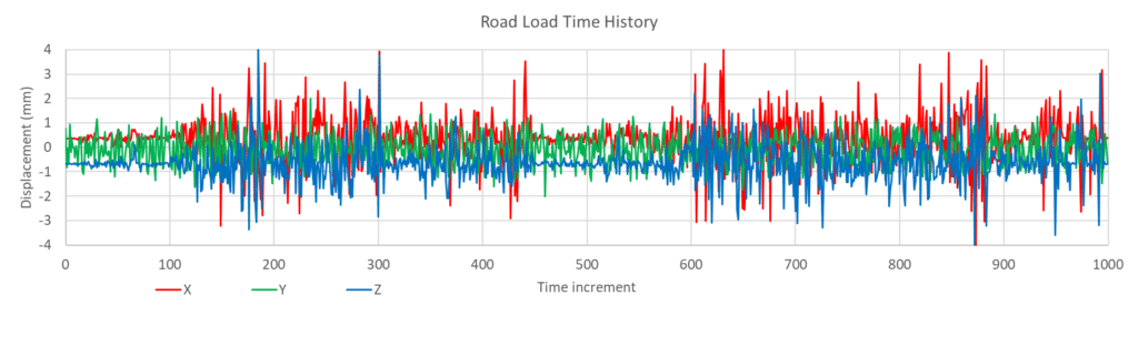
Let us dive into the process of block cycle creation using an example of a bushing and a road load history. The road loading history shown below contains results for loadings in 3 axes over a time history.

Road Load Time History Graph

The first step in creating the block cycle schedule is solving for the strain history over the entire road load history. Fortunately, Endurica EIE comes to the rescue in solving for the long strain history. The road load time history does not need to be modeled directly in FEA. Instead, a map is run in FEA to solve for strain history within the bounds of the road loading. Endurica EIE quickly interpolates the strains from this map to create the full loading strain history. In the animation below the map points solved for in FEA are shown as black dots and the bushing traces out the path of the map.

Endurica EIE quickly interpolating the strains from this map to create the full loading strain history

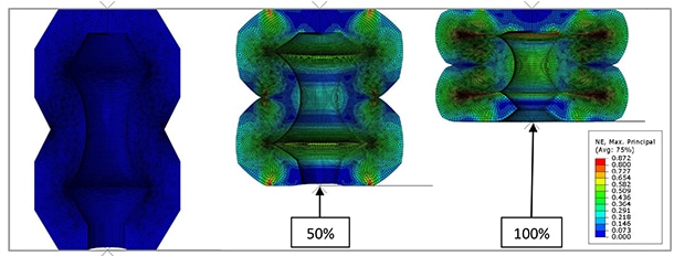
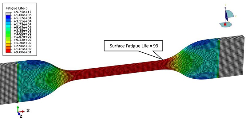
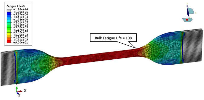
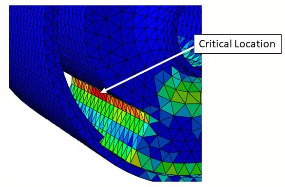
After the full road load strain history has been solved for in EIE the fatigue life for the road load signal is ready to be analyzed in CL. The fatigue analysis of the entire road load signal gives valuable insight into finding the critical location, developing the block cycle, and allowing the fatigue life of the block schedule to be validated against the fatigue life of the road load. The critical location of the bushing is shown in the image below:

The fatigue analysis of the entire load signal shows the critical location along with an estimated fatigue life

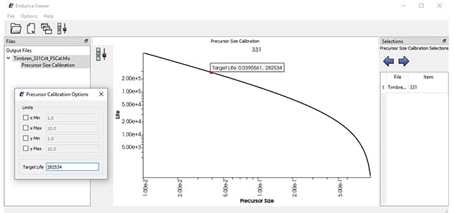
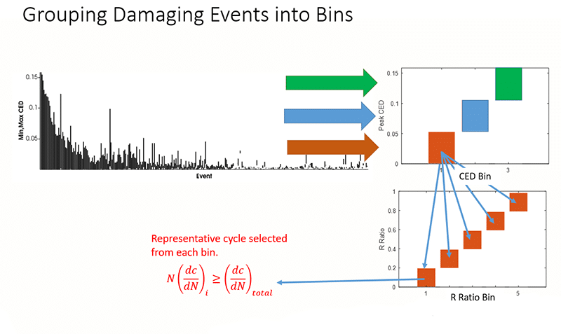
At the bushing critical location, all damaging events on the critical plane are taken into account when creating the block cycle schedule. The events are grouped into different bins categorized by two parameters: the peak CED and R ratio. The analyst remains in control by selecting the number of bins to group into. Each of the bins contains events with similar peak CED and R ratio that falls within the bounds of the bin. Within each bin, a representative cycle is identified that when repeated in the block schedule will contribute at least as much damage as all the various events in the bin. This selection process produces a conservative result that ensures that the block cycle will be at least as damaging as the road load.

Grouping Damaging events into Bins

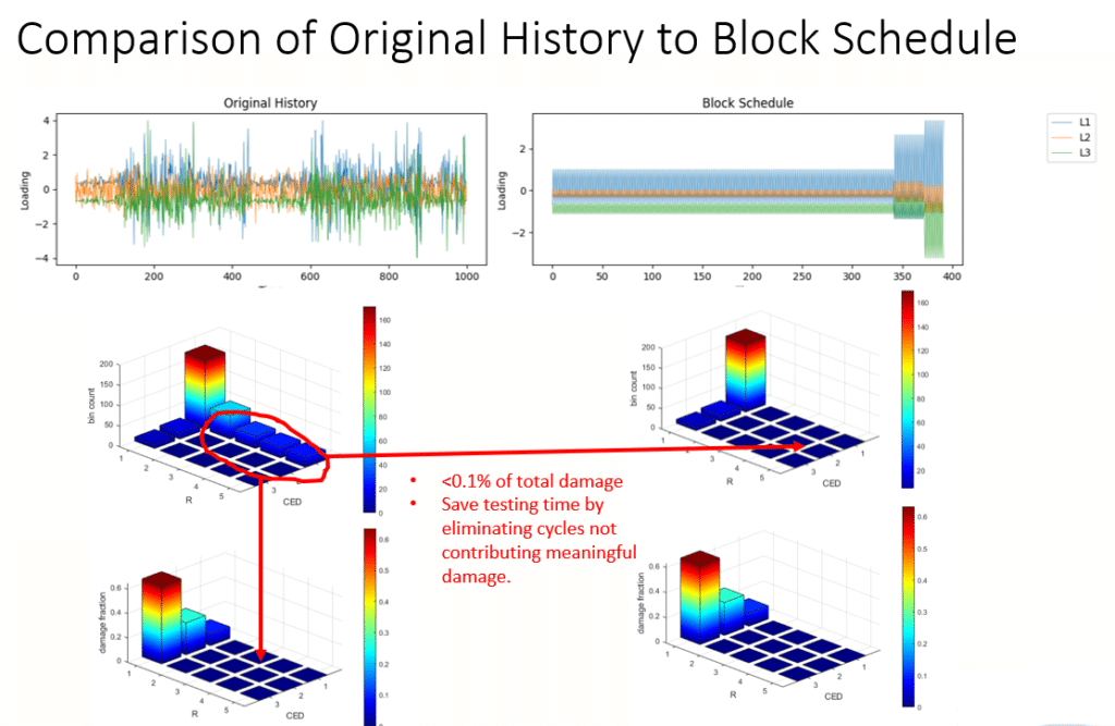
The bin results from the original history show the number of times each bin is repeated and the total damage from each bin. At this point, the bins that contribute insignificant damage can be safely eliminated from the block cycle schedule to save testing time and complexity without changing the results.

Comparison of Original history to Block Schedule

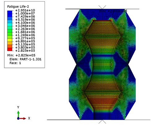
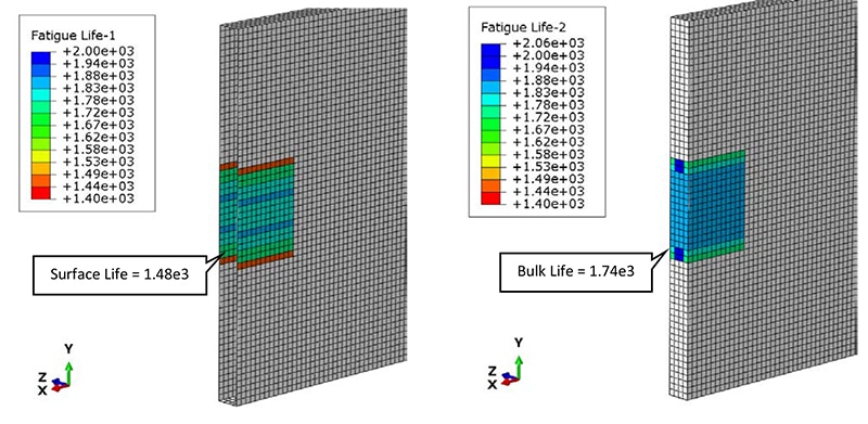
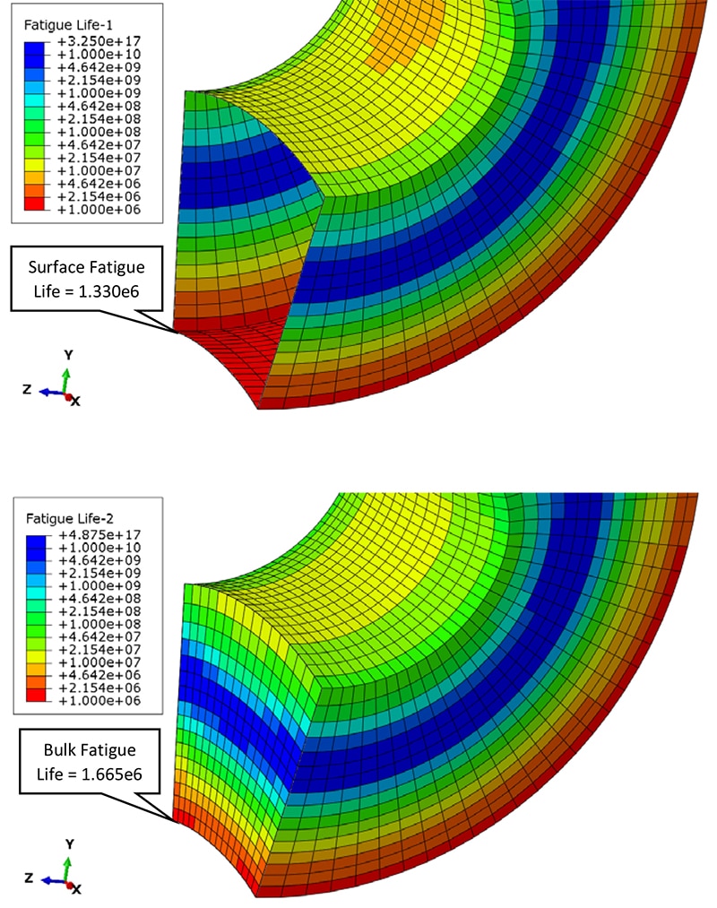
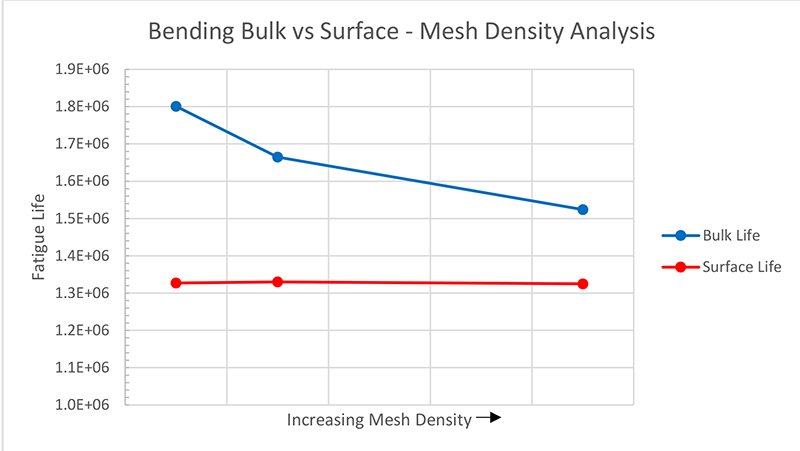
The simplified block schedule is then modeled to check the fatigue life vs the full road load signal. The results show that the critical location and fatigue life has been accurately maintained in the block schedule.

Road Load vs. Block Cycle Fatigue + Damage Spheres

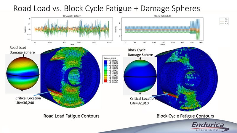
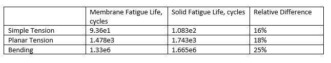
This automated block cycle creation procedure succeeded in producing a block cycle with the same critical location and very similar fatigue life. The block cycle selection was able to re-create the full road load signal using only three different loading blocks.

Endurica CL automated block cycle creation lets you take the guesswork out of block cycle creation and harness the proven power of Endurica fatigue analysis technology to get durability right.

Calibrating Crack Precursor Size in Endurica CL

June 6, 2022July 22, 2019 by Mark Bauman

Crack precursors exist in all elastomers owing to the heterogeneous microstructure, even before any loads are applied. The size of the typical precursor must be specified as part of the Endurica fatigue analysis workflow. The best practice for finding the precursor size is to leverage both crack growth and crack nucleation experiments to enforce agreement between the nucleation test results and the corresponding simulation-predicted life results. This procedure guarantees that both the crack growth and the crack nucleation experiments add up to an overall consistent story.

Prior to performing the calibration, you will need to have already defined the hyperelastic law, and the fatigue crack growth rate law. Fatigue models used for rubber have the following parameters:

Relationship between tearing energy and crack growth rate
- The parameters needed to define this relationship are obtained through fatigue crack growth experiments. The crack is loaded under a range of tearing energies while tracking growth of the crack. These tests obtain the critical tearing energy, T_c, which is the tearing energy at which the crack reaches end of life failure in one loading. The crack growth rate at critical tearing energy, r_c, and the slope of the curve, F, are determined by fitting a power law to the experimental crack growth and tearing energy.
Threshold
- This is the tearing energy limit T₀ below which cracks do not grow. If you do not specify this parameter, then you will use the Thomas law. If you do specify this parameter, you will use the Lake-Lindley law. The threshold can be measured using an Intrinsic Strength experiment.
Strain Crystallization
- Some rubbers exhibit a strain crystallization behavior that causes an increase of durability under non-relaxing loads. If the duty cycle of your calibration experiment is nonrelaxing, and if you have a strain crystallizing material, then this characterization should be completed before calibrating the precursor size. The strain crystallization effect is measured in the non-relaxing module.
End of life crack size
- This parameter should be set in the material definition prior to calibrating the precursor size. A default value of 1mm is generally adequate, particularly when it turns out that the precursor size is at least 5x smaller than this value. The part is considered to have failed when a crack reaches this size.

The crack nucleation experiment used for the calibration procedure may be made on a material test coupon, or on an actual component. Test coupons are convenient in early development stages as they do not require having a part to test. So long as crack precursor size is controlled by intrinsic features of the compound recipe (and not by the extrinsic features of post-mixing processes), a test coupon is likely to give useful results. There is a risk when using a test coupon: the risk that the precursor size in a manufactured part is actually controlled by some feature of post-mixing process such as factory contamination, part molding, abrasion, etc. This risk can be mitigated by calibrating precursor size on the basis of crack nucleation experiments on the finished part. In the following example, we show the process for calibration based on a finished part. The process for a test coupon is the same, but the model of the part is replaced by a model of the specimen.

To illustrate, take the case of a rubber bumper spring. Its duty cycle consists of compressing the 150 mm long rubber spring by 80 mm. Experiments show a fatigue life of 282,534 cycles for this duty cycle. A finite element analysis of the rubber spring is made to obtain strain history. The rubber spring is shown in the image below at the initial condition, at 50% of the displacement, and at 100% of the displacement during the fatigue duty cycle.

The rubber spring at the initial condition, at 50% of the displacement, and at 100% of the displacement during the fatigue duty cycle

We are now ready to calibrate the as yet unknown precursor size to the known experimental fatigue test result of the spring. The precursor size can be calibrated by calculating the fatigue life for a series of precursor sizes and then interpolating to find the one precursor size that results in the best agreement between fatigue life calculations and the experimental fatigue life. Use the PRECURSORSIZE_CALIBRATION output request in Endurica CL to produce a table of fatigue life vs. crack precursor size. Your output request syntax will look something like this:

**OUTPUT

PRECURSORSIZE_CALIBRATION, NFS=25, FSMIN=1e-2
LIFE

NFS is the number of precursor sizes to evaluate, in this case 25. FSMIN is the smallest precursor size to evaluate, in this case 0.01 mm.

Once you’ve executed the calibration, use the new Endurica Viewer to complete the calibration workflow. It can plot a wide range of Endurica analysis outputs including precursor size calibration. Just open the Endurica output file containing the calibration results and expand the output file contents tree to find the Precursor Size Calibration results. The viewer then plots the computed table of precursor size vs fatigue life.

The viewer plots the computed table of precursor size vs fatigue life

If you click on the plot options in the upper left corner, you can input the target life and the viewer will interpolate the precursor size. In this case, for a life of 282,534 cycles, the corresponding precursor size is 39 microns. Now that the precursor size is calibrated, the spring geometry can be optimized, different loadings analyzed, or entirely different parts can be analyzed using the material model to get fatigue life results that accurately reflect the precursor size that is most representative of the final material in the part. Again, if a part is not available, precursor size can also be calibrated to fatigue results from standard simple tension test specimen.

The calibrated rubber spring FE model with the life result of 282,534 cycles is shown below.

Fatigue Life Analysis of Free Surfaces

February 8, 2018February 1, 2018 by Mark Bauman

Free surfaces are critical in fatigue analysis because cracks in a physical part tend to form and grow fastest on such surfaces. Extra care is required when analyzing free surfaces because typical 3D solid finite elements have their worst accuracy at the free surface (gauss points are not located on the free surface, and hydrostatic pressure profile does not conform adequately to element shape function). Fortunately, the problem is not hard to resolve: free surfaces can easily be skinned with membrane elements. Membrane elements are specially formulated to produce an exact state of plane stress.

Let’s look at fatigue life predictions that have been computed with a skin of membrane elements, and compare them with predictions computed from the underlying 3D solid elements.

To study the differences in fatigue life calculations, three simple loading cases were used: simple tension, planar tension, and bending. For each case the fatigue life is calculated for both the surface and solid elements. The results are shown in the table below.

The fatigue life results show that the shortest life always occurred on the free surface. The life for the solid elements varied from 16% to 25% longer than the surface elements. In each case, the critical failure location was on the surface of the part and in the same location for both the solid and surface calculations. The colored contours of fatigue life are shown below for each of the cases.

Figure 1. Fatigue life on simple tension specimen. Isometric view.

Figure 2. Fatigue life on planar tension specimen. Cross-section view through the center of the specimen.

Figure 3. Fatigue life on bending specimen. Cross-section view through the center of the specimen.

Mesh refinement affects the fatigue life results. A mesh refinement study was performed on the bending case. The mesh refinement study consists of the standard mesh model shown above, a coarse mesh model and a fine mesh model. The number of elements in each model triples with each increase in mesh density. The results are shown below.

Figure 4. Mesh Density Analysis on bending specimen.

This mesh density analysis shows that as mesh density increases, the difference in the bulk and surface results decreases. The bulk and surface results converge to a single value. The amount that solid elements on the surface of the part extend into the interior of the part decreases as smaller elements are used. Since the smaller solid elements have a strain history closer to the surface they more closely match the surface element strains and the life results converge to a single value.

Bottom Line: if you have free surfaces, skin your model with membrane elements for high accuracy results. Refining your mesh at the surface may help somewhat, but skinning with membranes is far more reliable.