
Dr. Will Mars, founder and president of Endurica, challenged attendees to think beyond traditional boundaries and consider the many “Dimensions of Durability” that define product... Continue reading
Return to previous page
Tag: accuracy
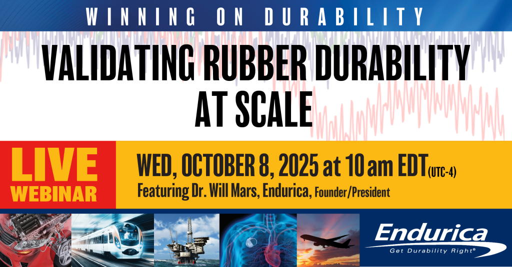
Discover how industry leaders are transforming their durability programs by simulating real-world road loads for rubber parts. This webinar features a verification and validation project... Continue reading
William V. Mars, Ph.D., P.E. is a co-author of the article A Preliminary Conceptual Study for Coupled Thermo-Mechanical and Structural Characterization of Rim-Supported Run-Flat Tires which... Continue reading

Rubber durability isn’t just a detail — it’s the difference between success and failure — especially in the rail industry. That’s why Endurica’s Winning on... Continue reading
It was May of 2023, and Will Mars had just given a presentation on “Virtual Qualification of the Durability Performance of an Elastomeric Mount with... Continue reading

All materials are temperature dependent, but some more than others: metals tend to be crystalline solids and will melt at sufficiently high temperatures; in contrast,... Continue reading

Wow – this year has really been one of many firsts for Endurica. We had our first ever Community Conference in April, we started our... Continue reading

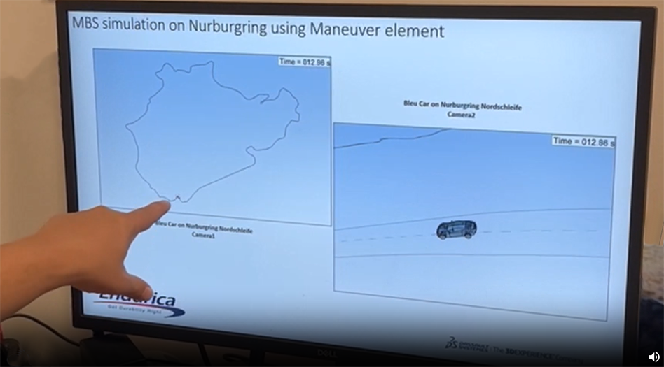
The load cases to be considered in fatigue analysis can be very lengthy and can involve multiple load axes. Often, load cases are much longer... Continue reading
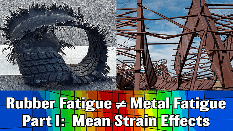
Rubber and metal are very different materials that exhibit very different behaviors. Consider the effect of mean strain or stress on the fatigue performance of... Continue reading

I get this question a lot: how well can the Endurica software predict fatigue life? Is it as good as a metal fatigue code, where... Continue reading
Showing 1–10 of 16 posts