The New Endurica Architecture – It’s Time to Migrate

Our transition to a new software architecture is a vital move in navigating the dynamic technological landscape. In a recent webinar, we discussed the aspects of this transition, providing insights into the why and how of adopting a new architectural approach despite having a functional existing one. This post will highlight the motivations behind the shift, the present status of feature migration, alterations in the latest software release, and an overview of projects within this new framework.

The Rationale and Benefits

Why Overhaul?

The complete rewrite of our software’s architecture was not a decision made lightly. The reasoning extends beyond merely wanting a refresh; it was driven by pivotal motivations, primarily surrounding the necessity for speed and efficiency in executing computing processes. Speed is invariably tied to productivity and operational fluency in software and technology. The plot below illustrates a compelling story: the old architecture (represented by the blue line), exhibited a static runtime, regardless of the number of threads engaged, revealing its inability to utilize parallel processing. Contrastingly, the new architecture demonstrates a significant speed-up, even with just a single thread, and scales to allow an increase in speed by many multiples, contingent on thread capacity.

Solving Larger Problems

The pursuit of faster execution isn’t arbitrary; it is intrinsically linked to our objective of solving larger problems. With larger tasks and projects on the horizon, scaling up and utilizing more CPU threads became essential. Exemplified through a job run on a virtual machine with 96 available CPU threads, the linear decrease in runtime with increasing threads (until certain hardware limitations are met) exhibits the new architecture’s adept handling of larger jobs (see plot below). The capability to scale and manage tasks of escalating complexity and size was a crucial driver for our transition.

Enhancing Integrations and Streamlining Workflows

Then, we turned our attention toward improving the user experience in interfacing with our software. Our prior use of the HFI and HFO file formats, while functional, presented numerous challenges regarding modification and integration, particularly when scripted modifications were necessary. The new architecture employs the JSON file format, widely recognized for its robustness and versatility across various industries and applications. With JSON, modifying job inputs and managing data become significantly simplified, as illustrated by a Python script example, wherein the entirety of job modifications, inputs, and submissions can be seamlessly handled with a handful of lines of code.

Improved Usability and Real-Time Error Checking

In an effort to enhance usability and mitigate the common issue of erroneous entries and syntax use, the new architecture, especially when utilized with a text editor like VS Code, offers real-time checking and syntax suggestions. This not only makes job submission more precise but also substantially reduces the trial-and-error cycle, saving valuable time. Additionally, upon job submission, the new architecture performs rigorous error and syntax checks, ensuring smooth execution and user experience.

Comprehensive Feature Migration: A Successful Transition

Reflecting on the past two years, we have accomplished a near-complete feature migration to the new software architecture, with 99% of features now successfully transitioned. This includes all outlined output requests, material models, history types, and various procedures.
Our commitment to supporting multiple interfaces remains, with support for Abaqus, Ansys, and Marc using the new architecture. Furthermore, Endurica Viewer is fully compatible, providing enhanced visualization capabilities under the new system.
The comprehensive migration and the incorporation of new functionalities marks the new architecture as fully operational and ready for use across all undertakings.

Implementation of Directory and Execution Changes in Endurica Software

Refined Directory Structure

In efforts to provide a seamless transition and user experience with the upgraded Endurica software, modifications have been made to the directory structure. The new architecture, once labeled “Katana” during its development phase, has now been ubiquitously integrated into the top-level Endurica directory. With the most recent software installation, users will observe the top-level CL and DT directories contain the new architecture, and the Katana directory has been removed.

Consequently, when we refer to Endurica CL and Endurica DT moving forward, it denotes reference to the new architecture.

Accommodating Transition: The Legacy Folder

Acknowledging that the transition to the new architecture may not be instantaneous for all users, the old architecture will still be available and designated within a “Legacy” folder. Though it requires navigation into subfolders, we ensure its accessibility for users who need more time to transition fully into the new structure.

Executable Naming Conventions

In tandem with the directory adjustments, executable naming conventions have been revised to be more intuitive. Previously, “endurica” was employed to submit fatigue analyses in the old architecture, while “katana” pertained to the new. To streamline, “katana” has been rebranded as “endurica” for submitting the JSON input file, with the legacy version adopting the name “endurica-legacy.” It is crucial to note that users accustomed to utilizing “katana” may continue to do so — “endurica” and “katana” will run the same executable. However, usage of the old architecture requires invoking a new “endurica-legacy” command.

Delivering the Unattainable with Endurica’s New Software Architecture

Embarking upon two recent projects with our new computational architecture, we explored the realms of virtual simulation and data management in tire durability and elastomeric mount durability performance.

Project 1: Tire Durability with Dassault Systems

In collaboration with Dassault Systems, a multi-body dynamic simulation was conducted to compute tire durability at the Nurburgring circuit. Utilizing SIMPACK for generating virtual road load data and employing Endurica EIE and Abaqus to establish a workspace map of driving conditions, the endeavor yielded significant data, processed through 176,000 time steps to evaluate the tire’s fatigue life. After a meticulous analysis, the results spotlighted the fatigue life to be 214 laps, pinpointing the most critical point around the tire bead edge.

Project 2: Durability of an Elastomeric Mount with Ford

Undertaken with Ford, the second project navigated through the durability performance of an elastomeric mount, involving a behemoth of data from 144 load history files, each load file containing tens or hundreds of thousands of time points, accumulating to over 15 million total time points. Utilizing a similar approach as the Nurburgring project, Endurica EIE and Abaqus were used together to generate the strain history data. The analysis focused on membrane elements on the mount’s free surfaces to precisely gauge surface strains. Culminating the analysis, the project succeeded in qualifying the part with a fatigue life of 9.4 repeats of the entire schedule, wherein the requisite was just one repeat.

These projects underscored the capabilities of our new architecture, navigating through large data sets and providing tangible insights in significantly reduced timeframes compared to the old architecture. In essence, the implementation of the new architecture has not only streamlined our processes but also expanded our horizons in handling large data and achieving nuanced analyses in our projects.

Summary

The new Endurica CL and Endurica DT architectures have now fully replaced our old system, maintaining the accuracy our users expect while introducing an easier, more powerful, and scalable solution. Everything has been successfully migrated over to this complete solution. With its enhanced capabilities, it addresses problems that were previously too large or took too long to solve, enabling our customers to tackle challenges they might not have considered before. The ability to solve unprecedented problems is just one more example of our steadfast commitment to providing accurate, complete, and scalable solutions.

twitterlinkedinmail

License Queueing

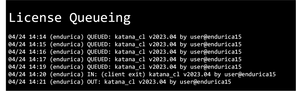
Design optimization studies are driving a need to support the efficient management and execution of many jobs.  This is why we are announcing that Endurica’s software license manager now supports queueing for licenses. This allows a submitted job to automatically wait to start until enough licenses are available, instead of the prior behavior of exiting with a license error. Now you can submit many jobs without worrying about license availability.

License queueing is only available for network licenses (not node-locked). It is currently supported for Katana CL/DT jobs and EIE jobs submitted from a command prompt.

To enable queueing, set the environment variable RLM_QUEUE to any value. This environment variable must be set on the client machine (not the license server).

To learn more about license queueing, search for “How to Queue for Licenses” in the RLM License Administration documentation here: https://www.reprisesoftware.com/RLM_License_Administration.pdf


twitterlinkedinmail

Endurica 2019 Updates Released

Endurica CL

Endurica CL received many improvements over the past year.  These improvements cover a wide variety of different aspects of the software:

Reducing Run-time

Our investments in code benchmarking and performance are paying off! We’ve been able to make internal optimizations to the code that reduce analysis run-times by approximately 30%. 

HFM and HFO Formatting

To make our output cleaner and more meaningful, small changes have been made to the number formatting in the HFM and HFO files.

All results reported in scientific notation are now formatted in standard form where the leading digit before the decimal point is non-zero (previously the leading digit was always zero).  This gives one more significant figure to all the results without increasing the output file size.

Signal compression

The shortest fatigue life for the analysis is now printed to the console and HFM file with six significant figures.  Previously, the life was reported with only two significant figures.  This change makes it easier to quickly compare two different analyses, especially when the analyses have similar fatigue lives.

New features have been added to Endurica CL to make it easier to process and analyze histories.  Using the new COMPRESS_HISTORY output request, you can generate new HFI files containing compressed versions of your original history.  The generated history is composed of the rainflow counted cycles from your original history.  An optional output parameter allows you to further compress the signal by specifying the minimum percentage of the original damage that should be retained in the new history.  When keeping a percentage of the damage, the cycles are sorted from most to least damaging so that the generated history always contains the most damaging cycles and discards the least damaging cycles.

This output request is useful when you want to reduce a long complex history while keeping the important damaging cycles.  This can reduce file sizes and simplify experimental testing setups as well as give you a deeper insight into your duty cycle. 

Endurica DT

Endurica DT is our incremental fatigue solver.  With Endurica CL, your analysis starts at time zero and integrates the given strain history until end-of-life.  With Endurica DT, you can start and end at a series of times that you specify.  This lets you accumulate many different histories and loading conditions repeatedly until end-of-life.

With Endurica DT, it allows you to start and end at a series of times, when specified.

Endurica DT gives you new ways to control your analyses, and we have been using it over the past year in many applications.  For example, fatigue results for laboratory test procedures that involve multiple loading stages (such as FMVSS No. 139 for light vehicle tires, or block cycle schedules for automotive component applications) can be fully simulated using Endurica DT. You can also compute residual life following some scheduled set of load cases. 

Endurica DT can also be used to accumulate the actual loads measured on a part in situ.  This allows you to create a digital twin that keeps a near real-time record of the part’s current simulated damage state and the part’s remaining fatigue life. 

Stiffness Loss Co-Simulation

Endurica DT now includes a stiffness loss co-simulation workflow that allows you to iteratively update the stiffness of your part over a series of time steps, based on the amount of damage occurring in the part.  The stiffness loss is computed per element so you will have a gradient where the more damaged regions become softer.  Endurica DT computes the current fraction h of stiffness loss based on the stress and strain, and the finite element solver computes the stress and strain based on the current fractions of stiffness loss. The capability accurately predicts the effects of changing mode of control during a fatigue test.  For example, stress controlled fatigue tests show shorter life than strain controlled fatigue tests. 

Endurica DT now includes a stiffness loss co-simulation workflow

Endurica EIE

Endurica EIE, our efficient interpolation engine, quickly generates long, complex histories using a set of precomputed finite element results (i.e. the ‘nonlinear map’).  We first launched EIE last year with the ability to interpolate 1-channel and 2-channel problems.  We have recently added the ability to interpolate 3-channel problems. 

In the example below, EIE was benchmarked with three-channels.  Three separate road load signals were computed from a single nonlinear map.  With EIE, you don’t need to rerun the finite element model for each history.  Instead, EIE interpolates from the nonlinear map, providing the equivalent results with a 60x speed-up in compute time. 

Endurica EIE interpolates from the nonlinear map, providing the equivalent results
twitterlinkedinmail

Behind the Scenes Tour of Endurica Software Development and QA Practices

Ever wonder what it takes to consistently deliver quality and reliability in our software releases?  Here’s a brief overview of the systems and disciplines we use to ensure that our users receive timely, trouble-free updates of Endurica software.

Automation:

Throughout the life of our software, changes are made to our source code for a variety of reasons.  Most commonly, we are adding new features and capabilities to our software.  We also make updates to the code to improve performance and to squash the inevitable bugs that occasionally occur.

With each change committed to the code repository, the software needs to be built, tested, and released.  Endurica’s workflow automates these steps so that any change to the source repository triggers a clean build of the software.  A successful build is automatically followed by a testing phase where our suite of benchmarks is executed and compared to known results.  Finally, the build is automatically packaged and stored so that it is ready to be delivered.  At each step along the way, a build error or failed test will cancel the workflow and send an alert warning that the release has been rejected, so that the issue can be addressed, and the workflow restarted.

Endurica's build and testing process ensures that high quality standards are met for every new release. Black arrow: normal flow, Red arrow: an error or failed test
Figure 1: Endurica’s build and testing process ensures that high quality standards are met for every new release. Black arrow: normal flow, Red arrow: an error or failed test.

Reliability:

The automated testing phase that every release goes through helps ensure the reliability of our software.  For example, every Endurica CL release must pass all 70 benchmarks.  Each benchmark is a separate Endurica CL analysis made up of different materials, histories, and output requests.  Results from a new build are compared to known results from the previous successful build.  If results do not agree, or if there are any errors, the benchmark does not pass and the build is rejected.

The testing phase prevents “would-be” bugs from making it into a release and makes sure that any issues get resolved.

Repeatability:

The automated nature of our development workflow naturally helps with repeatability in our releases.  Each build flows through the same pipeline, creating consistent releases every time.  There is less worry, for example, that a component will be forgotten to be included.  It also allows us to recreate previous versions if comparisons need to be made.

Traceability:

Our version control system enables us to easily pinpoint where and when prior changes were introduced into the software.  Each release is tied to a commit in the repository. This allows any future issues to be easily traced back and isolated to a small set of changes in the source for quick resolution.

Responsiveness:

Automating the build and release pipelines greatly increases our responsiveness.  If an issue is discovered in a release, the problem can be resolved, and a fully corrected and tested release can be made available the same day.  We can also quickly respond to user feedback and suggestions by making small and frequent updates.

The systems and disciplines we use in our development process make us very efficient, and they protect against many errors. This means we can spend more of our time on what matters: delivering and improving software that meets high standards and helps you to get durability right.twitterlinkedinmail

EIE – Effect of Map Discretization on Interpolation Accuracy

Overview

The accuracy of the interpolated results performed by EIE is dependent on the discretization of the map. Specifically, the results will become more accurate as the map’s point density increases. This study uses a simple 2D model to quantify the accuracy of results interpolated from maps with different densities.

Model

A 1 mm x 1 mm rubber 2D plane strain model with two channels is used. The square’s bottom edge is fixed and the top edge is displaced in the x and y directions as shown below. The x displacement corresponds to channel 1 and the y displacement corresponds to channel 2. The working space of the model is defined by the x displacement ranging from 0 mm to 0.8 mm and the y displacement ranging from -0.08 mm to 0.8 mm.

Plane strain model with two channels

The model is meshed with 100 8-node, quadrilateral, plane strain, hybrid, reduced integration elements (shown below).

100 element mesh
100 element mesh

History

We define as the benchmark reference solution a history that covers the model’s entire working space with a high density of points. An evenly spaced grid of 128×128 points for a total of 16384 points is used as the history (shown below). It is important that this history is more refined than the maps that we will create to ensure that we are testing all regions of our maps.

128 x 128 history points
128×128 history points

These points are used to drive the finite element model and the results are recorded. For this study, we record the three non-zero strain components and the hydrostatic pressure (NE11, NE22, NE12, and HP) for each element at each time point. In summary, there are 4 result components, 100 elements, and 16384 time increments. This set of results is the reference solution since it is solved directly by the finite element model. We will compare this solution to our interpolated results to measure our interpolation accuracy.

Maps

Six maps with different levels of refinement are used to compute interpolated results for our history points. All of the maps structure their points as an evenly spaced grid. The first map starts with two points along each edge. With each additional map, the number of points along each edge is doubled so that the sixth and final map has 64 edge points. The map points for the six maps are shown below.

Six maps with increasing levels of refinement, structuring their points on an evenly spaced grid
Six maps with increasing levels of refinement

The map points for these six maps are used to drive the finite element model’s two channels. The strain and hydrostatic pressure results from the FEA solutions are recorded at each map point in a similar way to how the results were recorded for the FEA solution that was driven by the history points. Next, EIE is used six times to interpolate the map point results at each resolution onto the high resolution reference history points.

We now have seven sets of history results: the true set of results and six interpolated sets of results.

Results

To compare our results, we look at the absolute difference between the sets of results. The absolute error is used, opposed to a relative error, since some regions of the model’s working space will give near zero strain and hydrostatic pressure. Division by these near zero values would cause the relative error to spike in those regions.

Since we have 100 elements and 4 components per element, there are a lot of results that could be compared. To focus our investigation, we look at the element and component that gave the maximum error. The figure below shows contour plots for each of the six maps for this worst-case element and component. The component that gave the maximum error was NE12. The title of each of the contour plot also shows the maximum error found for each of the plots.

Error contours for the worst-case element and component. Titles report the maximum log10 error.

You can see that the error decreases as the map density increases. Also, you can identify the grid pattern in the contour plots since the error gets smaller near the map points.

Plotting the maximum error for each of the maps against the number of map points on a log scale is shown below. The slope of this line is approximately equal to 1 which is expected since a linear local interpolation was used to compute the results.

Maximum error vs the number of points for each of the six maps
twitterlinkedinmail

Specifying Strain Crystallization Effects for Fatigue Analysis

Endurica CL and fe-safe/Rubber provide several material models for defining cyclic crack growth under nonrelaxing conditions.  Nonrelaxing cycles occur when the ratio R is greater than zero.  R is defined as

R = (T min)/(Tmax)

where T is the energy release rate (note that T will always be greater than or equal to zero).

The crack growth rate under nonrelaxing conditions is, in general, a function of both Tmax and R. For purposes of calculation, it is convenient to define an “equivalent” energy release rate Teq that gives the same steady state rate of crack growth as the operating condition on the nonrelaxing crack growth curve, but which is instead on the fully relaxing crack growth curve.  In other words,

f(Teq) = f(Tmax, R).

Using this scheme, you can set up models for both amorphous and strain-crystallizing rubbers, depending on your definition of Teq.  Amorphous rubbers follow the well-known Paris model, and strain-crystallizing rubbers follow the Mars-Fatemi model (or you can define a lookup table).

Paris Model (Amorphous):

The Paris model is the simplest to derive, as it does not involve any material parameters.  It defines the equivalent energy release rate as

Teq = ∆T = Tmax (1-R)

This definition is only suitable for rubbers that do not strain-crystallize.

For strain-crystallizing rubbers, one of the other two models should be used.

Mars-Fatemi Model (Strain-crystallizing):

The Mars-Fatemi model accounts for strain crystallization by treating the power-law slope, F, of the Thomas fatigue crack growth rate law   r = rc (Tmax/ Tc) ^ (F(R))as a function of R, where

F(R) = F0e^(F4R)

or

F(R) = F0 + F1R + F2R^2 + F3R3

The exponential version is more compact, but the polynomial version is more flexible.

By substituting F(R) into the fatigue crack growth rate equations for relaxing and nonrelaxing cases, and doing a bit of algebra, the following relationship is obtained

Teq (Tmax, R) = Tmax,R ^(F(R)/F(0)) Tc^(1-(F(R)/F(0)))


Lookup Table (Strain-crystallizing):

The most flexible and accurate way to define strain crystallization is via a lookup table.  The lookup table takes R as an input and returns x(R) as an output.  This function can be defined as the fraction x(R) by which the nonrelaxing crack growth curve is shifted between the fully relaxing crack growth curve (x=0), and the vertical asymptote at Tc (x=1), at a given R.

x(R) = (log(T) - log(Teq))/(log(Tc) - log(Teq))

This can be rearranged into the desired Teq (Tmax,R) form, as follows

Teq = (Tmax ^(1/1-x(R)) Tc ^-(x(R)/1-x(R)))

Comparisons:

Visualizing the differences between the models helps gain a better understanding of how strain crystallization can affect fatigue performance.  Since all of these models can be represented in the same form of Teq(Tmax,R), we show 2-D contour plots of Teq with R on the x-axis and ∆T on the y-axis.  ∆T is used instead of Tmax to make it easier to compare back to the simple Paris model.

2D contour plots of Teq with R on the x-axis and ∆T on the y-axis. ∆T is used instead of Tmax to make it easier to compare back to the simple Paris model.

From the figures above, we see that for the Paris model, the equivalent energy release rate depends only on ∆T.  When using this model, changes in R will have no effect on fatigue performance (when ∆T is also held constant).

For strain-crystallizing rubbers, changes in R should influence fatigue performance.  This is seen in the figures for the Mars-Fatemi and lookup table models.

The Mars-Fatemi example uses the following parameters:

Parameters used in the Mars-Fatmi example

The lookup table example uses Tc=10.0 kJ/m2 and Lindley’s data for unfilled natural rubber (P. B. Lindley, Int. J. Fracture 9, 449 (1973)).

For these models, there is a significant decline in Teq as R increases.  This effect is most pronounced when Tmax is much smaller than the critical energy release rate Tc.  Also, there is a point where the effect is reversed (around R=0.8 in these examples) and the high R-ratio starts to have a negative effect on fatigue performance.

Implications:

A material’s strain crystallization properties’ impact on fatigue performance under non-relaxing conditions should not be ignored.  Whether you are seeking to take advantage of strain-crystallization effects or simply comparing the results of different materials/geometries/loadings, strain-crystallization should be accurately represented in your simulations.

Follow these tips to take advantage of strain crystallization and help ensure your fatigue performance is the best it can be.

  • Take advantage of Endurica’s material characterization service (the FPM-NR Nonrelaxing Module generates the strain crystallization curve) or use your own in-house testing to create an accurate strain crystallization model of your material (the nonrelaxing procedure is available for the Coesfeld Tear and Fatigue Analyser).
  • Use output requests like DAMAGE_SPHERE, CEDMINMAX and CEDRAINFLOW to observe R-ratios for your duty cycles.


References

  1. B. Lindley, Int. J. Fracture 9, 449 (1973)

Mars, W. V. “Fatigue life prediction for elastomeric structures.” Rubber chemistry and technology 80, no. 3 (2007): 481-503.

Mars, W. V. “Computed dependence of rubber’s fatigue behavior on strain crystallization.” Rubber Chemistry and Technology 82, no. 1 (2009): 51-61.

Barbash, Kevin P., and William V. Mars. Critical Plane Analysis of Rubber Bushing Durability under Road Loads. No. 2016-01-0393. SAE Technical Paper, 2016.


 twitterlinkedinmail

close
Trial License RequestTrial License RequestTrial License RequestTrial License RequestTrial License Request

Our website uses cookies. By agreeing, you accept the use of cookies in accordance with our cookie policy.  Continued use of our website automatically accepts our terms. Privacy Center