
Endurica is committed to building long-term, strategic relationships that support our clients’ success well beyond the initial purchase of a software license. In response to... Continue reading
Return to previous page
Category: Software
William V. Mars, Ph.D., P.E. is a co-author of the article A Preliminary Conceptual Study for Coupled Thermo-Mechanical and Structural Characterization of Rim-Supported Run-Flat Tires which... Continue reading
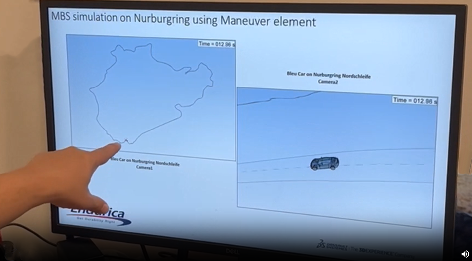
It was May of 2023, and Will Mars had just given a presentation on “Virtual Qualification of the Durability Performance of an Elastomeric Mount with... Continue reading

All materials are temperature dependent, but some more than others: metals tend to be crystalline solids and will melt at sufficiently high temperatures; in contrast,... Continue reading

Wow – this year has really been one of many firsts for Endurica. We had our first ever Community Conference in April, we started our... Continue reading
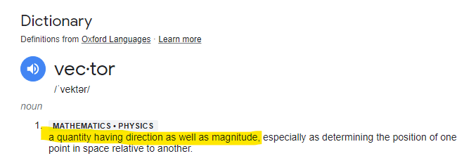
2023 marked year 15 for Endurica. If I had to pick one word to describe the past year, that word would be “vector”. Because magnitude... Continue reading
Our transition to a new software architecture is a vital move in navigating the dynamic technological landscape. In a recent webinar, we discussed the aspects... Continue reading
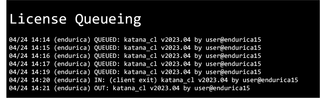
Design optimization studies are driving a need to support the efficient management and execution of many jobs. This is why we are announcing that Endurica’s... Continue reading
Expanded our team! We welcomed 35-year Goodyear veteran Tom Ebbott to our team as Vice President, and at one point we had 3 interns working... Continue reading
We’ve just added a new output to the Endurica fatigue solver: Safety Factor. This feature makes it simple to focus your analysis on whether cracks... Continue reading
Showing 1–10 of 15 posts