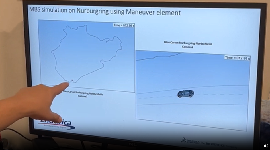
License Queueing

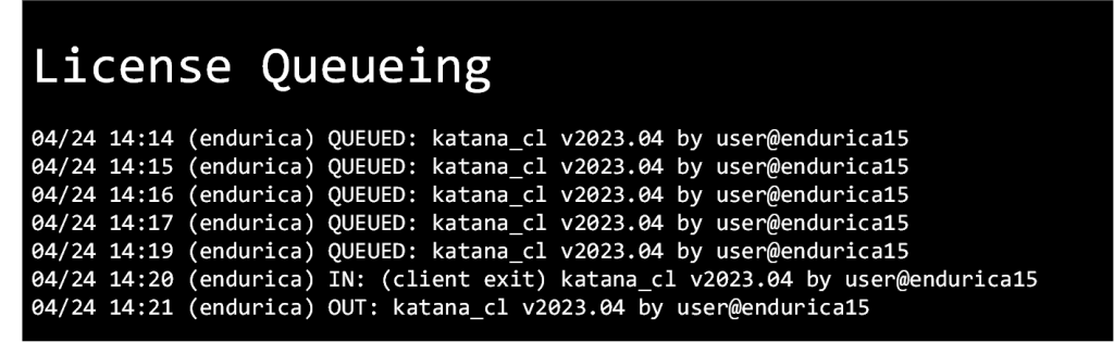
Design optimization studies are driving a need to support the efficient management and execution of many jobs.  This is why we are announcing that Endurica’s software license manager now supports queueing for licenses. This allows a submitted job to automatically wait to start until enough licenses are available, instead of the prior behavior of exiting with a license error. Now you can submit many jobs without worrying about license availability.

License queueing is only available for network licenses (not node-locked). It is currently supported for Katana CL/DT jobs and EIE jobs submitted from a command prompt.

To enable queueing, set the environment variable RLM_QUEUE to any value. This environment variable must be set on the client machine (not the license server).

To learn more about license queueing, search for “How to Queue for Licenses” in the RLM License Administration documentation here: https://www.reprisesoftware.com/RLM_License_Administration.pdf


twitterlinkedinmail

Road Loads to Block Cycle Schedule

 Road loads being converted into block cycle schedules through Endurica softwareRoad load signals are notoriously difficult to work with. The signals feature so many different time increments that it becomes too much to directly model efficiently in FEA. It is difficult to tell which portions of the loading do the most damage. Experimental fatigue testing would be too time-consuming and costly to run on the full complex road load signal. For these reasons simplifying road loads into block cycle schedules has become the gold standard for working with road load signals. Experimental testing and FEA modeling are more manageable when using a block cycle schedule instead of the full road load signal. Traditional methods of converting a road load signal to block cycle schedule can often fall short. Endurica recently added a built-in method in the Endurica CL software that uses the power of critical plane analysis and rain-flow counting to automate block cycle creation.

Let us dive into the process of block cycle creation using an example of a bushing and a road load history. The road loading history shown below contains results for loadings in 3 axes over a time history.

 Road Load Time History Graph

The first step in creating the block cycle schedule is solving for the strain history over the entire road load history. Fortunately, Endurica EIE comes to the rescue in solving for the long strain history. The road load time history does not need to be modeled directly in FEA. Instead, a map is run in FEA to solve for strain history within the bounds of the road loading. Endurica EIE quickly interpolates the strains from this map to create the full loading strain history. In the animation below the map points solved for in FEA are shown as black dots and the bushing traces out the path of the map.

Endurica EIE quickly interpolating the strains from this map to create the full loading strain history

After the full road load strain history has been solved for in EIE the fatigue life for the road load signal is ready to be analyzed in CL. The fatigue analysis of the entire road load signal gives valuable insight into finding the critical location, developing the block cycle, and allowing the fatigue life of the block schedule to be validated against the fatigue life of the road load. The critical location of the bushing is shown in the image below:

The fatigue analysis of the entire load signal shows the critical location along with an estimated fatigue life

At the bushing critical location, all damaging events on the critical plane are taken into account when creating the block cycle schedule. The events are grouped into different bins categorized by two parameters: the peak CED and R ratio. The analyst remains in control by selecting the number of bins to group into. Each of the bins contains events with similar peak CED and R ratio that falls within the bounds of the bin. Within each bin, a representative cycle is identified that when repeated in the block schedule will contribute at least as much damage as all the various events in the bin. This selection process produces a conservative result that ensures that the block cycle will be at least as damaging as the road load.

 Grouping Damaging events into Bins

The bin results from the original history show the number of times each bin is repeated and the total damage from each bin. At this point, the bins that contribute insignificant damage can be safely eliminated from the block cycle schedule to save testing time and complexity without changing the results.

Comparison of Original history to Block Schedule


The simplified block schedule is then modeled to check the fatigue life vs the full road load signal. The results show that the critical location and fatigue life has been accurately maintained in the block schedule.

 Road Load vs. Block Cycle Fatigue + Damage Spheres

This automated block cycle creation procedure succeeded in producing a block cycle with the same critical location and very similar fatigue life. The block cycle selection was able to re-create the full road load signal using only three different loading blocks.

Endurica CL automated block cycle creation lets you take the guesswork out of block cycle creation and harness the proven power of Endurica fatigue analysis technology to get durability right.

twitterlinkedinmail

Things that went right in 2020 at Endurica

Things that went right in 2020 at Endurica

2020 is burned in all our minds as a chaotic and tough year.  Just like the rest of the world, Endurica staff experienced times of isolation and loss due to the pandemic.  On a positive note, we invested heavily in making our tools and workflows better than ever so that we’re ready to come back strong in 2021.  Here is a list of our top new developments in 2020:

Endurica Software Enhancements

  • Endurica DT’s new Ageing Feature now enables you to simulate how ageing affects your rubber product. Your compound’s stiffness, strength, and fatigue properties can all evolve with time.
  • Our new Linux distribution takes our solutions beyond the Windows world.
  • We’ve added an encryption feature to safeguard your trade secrets.
  • Viewer Improvements make it easier than ever to visualize your fatigue simulation results.
  • EIE Enhancements give you blazing-fast compute speed for full road-load signals.
  • We’ve also planned an aggressive development agenda for 2021. Stay tuned for a new Endurica-based smartphone app for materials engineers, for a new feature that computes fatigue threshold safety margins, for a new block cycle schedule extraction algorithm, and more!

Training

  • The new Fatigue Ninja Friday webinar series provides step-by-step application training for key the workflows that you need to get durability right. All of the recorded episodes are now available in the online Endurica academy.
  • The new Winning on Durability webinar series provides high-level overviews of both technical and business topics so you can connect Endurica tools to your strategic imperatives. All of these recorded webinars are available gratis on our website.
  • We’ve recast our in-person training events as LIVE, ONLINE workshops accessible safely around the world.

Testing Instruments

Fatigue Property Mapping Testing Service

  • We added the Reliability Module to our Fatigue Property Mapping testing service. Use it to quantify crack precursor size statistics when you need to estimate probability of failure.
  • We also reorganized the Thermal Module and the Ageing Module into Basic and Advanced levels, to offer a lower price-point when a basic option will suffice.

Want to leverage any of these new capabilities in your next durability project?  Give us a call and let’s talk!

twitterlinkedinmail

Endurica 2019 Updates Released

Endurica CL

Endurica CL received many improvements over the past year.  These improvements cover a wide variety of different aspects of the software:

Reducing Run-time

Our investments in code benchmarking and performance are paying off! We’ve been able to make internal optimizations to the code that reduce analysis run-times by approximately 30%. 

HFM and HFO Formatting

To make our output cleaner and more meaningful, small changes have been made to the number formatting in the HFM and HFO files.

All results reported in scientific notation are now formatted in standard form where the leading digit before the decimal point is non-zero (previously the leading digit was always zero).  This gives one more significant figure to all the results without increasing the output file size.

Signal compression

The shortest fatigue life for the analysis is now printed to the console and HFM file with six significant figures.  Previously, the life was reported with only two significant figures.  This change makes it easier to quickly compare two different analyses, especially when the analyses have similar fatigue lives.

New features have been added to Endurica CL to make it easier to process and analyze histories.  Using the new COMPRESS_HISTORY output request, you can generate new HFI files containing compressed versions of your original history.  The generated history is composed of the rainflow counted cycles from your original history.  An optional output parameter allows you to further compress the signal by specifying the minimum percentage of the original damage that should be retained in the new history.  When keeping a percentage of the damage, the cycles are sorted from most to least damaging so that the generated history always contains the most damaging cycles and discards the least damaging cycles.

This output request is useful when you want to reduce a long complex history while keeping the important damaging cycles.  This can reduce file sizes and simplify experimental testing setups as well as give you a deeper insight into your duty cycle. 

Endurica DT

Endurica DT is our incremental fatigue solver.  With Endurica CL, your analysis starts at time zero and integrates the given strain history until end-of-life.  With Endurica DT, you can start and end at a series of times that you specify.  This lets you accumulate many different histories and loading conditions repeatedly until end-of-life.

With Endurica DT, it allows you to start and end at a series of times, when specified.

Endurica DT gives you new ways to control your analyses, and we have been using it over the past year in many applications.  For example, fatigue results for laboratory test procedures that involve multiple loading stages (such as FMVSS No. 139 for light vehicle tires, or block cycle schedules for automotive component applications) can be fully simulated using Endurica DT. You can also compute residual life following some scheduled set of load cases. 

Endurica DT can also be used to accumulate the actual loads measured on a part in situ.  This allows you to create a digital twin that keeps a near real-time record of the part’s current simulated damage state and the part’s remaining fatigue life. 

Stiffness Loss Co-Simulation

Endurica DT now includes a stiffness loss co-simulation workflow that allows you to iteratively update the stiffness of your part over a series of time steps, based on the amount of damage occurring in the part.  The stiffness loss is computed per element so you will have a gradient where the more damaged regions become softer.  Endurica DT computes the current fraction h of stiffness loss based on the stress and strain, and the finite element solver computes the stress and strain based on the current fractions of stiffness loss. The capability accurately predicts the effects of changing mode of control during a fatigue test.  For example, stress controlled fatigue tests show shorter life than strain controlled fatigue tests. 

Endurica DT now includes a stiffness loss co-simulation workflow

Endurica EIE

Endurica EIE, our efficient interpolation engine, quickly generates long, complex histories using a set of precomputed finite element results (i.e. the ‘nonlinear map’).  We first launched EIE last year with the ability to interpolate 1-channel and 2-channel problems.  We have recently added the ability to interpolate 3-channel problems. 

In the example below, EIE was benchmarked with three-channels.  Three separate road load signals were computed from a single nonlinear map.  With EIE, you don’t need to rerun the finite element model for each history.  Instead, EIE interpolates from the nonlinear map, providing the equivalent results with a 60x speed-up in compute time. 

Endurica EIE interpolates from the nonlinear map, providing the equivalent results
twitterlinkedinmail

EIE – Effect of Map Discretization on Interpolation Accuracy

Overview

The accuracy of the interpolated results performed by EIE is dependent on the discretization of the map. Specifically, the results will become more accurate as the map’s point density increases. This study uses a simple 2D model to quantify the accuracy of results interpolated from maps with different densities.

Model

A 1 mm x 1 mm rubber 2D plane strain model with two channels is used. The square’s bottom edge is fixed and the top edge is displaced in the x and y directions as shown below. The x displacement corresponds to channel 1 and the y displacement corresponds to channel 2. The working space of the model is defined by the x displacement ranging from 0 mm to 0.8 mm and the y displacement ranging from -0.08 mm to 0.8 mm.

Plane strain model with two channels

The model is meshed with 100 8-node, quadrilateral, plane strain, hybrid, reduced integration elements (shown below).

100 element mesh
100 element mesh

History

We define as the benchmark reference solution a history that covers the model’s entire working space with a high density of points. An evenly spaced grid of 128×128 points for a total of 16384 points is used as the history (shown below). It is important that this history is more refined than the maps that we will create to ensure that we are testing all regions of our maps.

128 x 128 history points
128×128 history points

These points are used to drive the finite element model and the results are recorded. For this study, we record the three non-zero strain components and the hydrostatic pressure (NE11, NE22, NE12, and HP) for each element at each time point. In summary, there are 4 result components, 100 elements, and 16384 time increments. This set of results is the reference solution since it is solved directly by the finite element model. We will compare this solution to our interpolated results to measure our interpolation accuracy.

Maps

Six maps with different levels of refinement are used to compute interpolated results for our history points. All of the maps structure their points as an evenly spaced grid. The first map starts with two points along each edge. With each additional map, the number of points along each edge is doubled so that the sixth and final map has 64 edge points. The map points for the six maps are shown below.

Six maps with increasing levels of refinement, structuring their points on an evenly spaced grid
Six maps with increasing levels of refinement

The map points for these six maps are used to drive the finite element model’s two channels. The strain and hydrostatic pressure results from the FEA solutions are recorded at each map point in a similar way to how the results were recorded for the FEA solution that was driven by the history points. Next, EIE is used six times to interpolate the map point results at each resolution onto the high resolution reference history points.

We now have seven sets of history results: the true set of results and six interpolated sets of results.

Results

To compare our results, we look at the absolute difference between the sets of results. The absolute error is used, opposed to a relative error, since some regions of the model’s working space will give near zero strain and hydrostatic pressure. Division by these near zero values would cause the relative error to spike in those regions.

Since we have 100 elements and 4 components per element, there are a lot of results that could be compared. To focus our investigation, we look at the element and component that gave the maximum error. The figure below shows contour plots for each of the six maps for this worst-case element and component. The component that gave the maximum error was NE12. The title of each of the contour plot also shows the maximum error found for each of the plots.

Error contours for the worst-case element and component. Titles report the maximum log10 error.

You can see that the error decreases as the map density increases. Also, you can identify the grid pattern in the contour plots since the error gets smaller near the map points.

Plotting the maximum error for each of the maps against the number of map points on a log scale is shown below. The slope of this line is approximately equal to 1 which is expected since a linear local interpolation was used to compute the results.

Maximum error vs the number of points for each of the six maps
twitterlinkedinmail

close
Trial License RequestTrial License RequestTrial License RequestTrial License RequestTrial License Request

Our website uses cookies. By agreeing, you accept the use of cookies in accordance with our cookie policy.  Continued use of our website automatically accepts our terms. Privacy Center